Wednesday 12 December 2018

VTU PYTHON SYLLABUS

Module – 1 : Why should you learn to write programs, Variables, expressions and statements, Conditional execution, Functions –8Hours
Module – 2 : Iteration, Strings, Files –8 Hours
Module – 3 : Lists, Dictionaries, Tuples, Regular Expressions–8 Hours
Module – 4 : Classes and objects, Classes and functions, Classes and methods–8 Hours
Module – 5 : Networked programs, Using Web Services, Using databases and SQL–8 Hours

Course objectives: This course will enable students to
Learn Syntax and Semantics and create Functions in Python.
Handle Strings and Files in Python.
Understand Lists, Dictionaries and Regular expressions in Python.
Implement Object Oriented Programming concepts in Python
Build Web Services and introduction to Network and Database Programming in Python.

Course outcomes: The students should be able to:
Examine Python syntax and semantics and be fluent in the use of Python flow control and functions.
Demonstrate proficiency in handling Strings and File Systems.
Create, run and manipulate Python Programs using core data structures like Lists, Dictionaries and use Regular Expressions.
Interpret the concepts of Object-Oriented Programming as used in Python.
Implement exemplary applications related to Network Programming, Web Services and Databases in Python.

Question paper pattern:
The question paper will have TEN questions. There will be TWO questions from each module. Each question will have questions covering all the topics under a module. The students will have to answer FIVE full questions, selecting ONE full question from each module.

Text Books:
1. Charles R. Severance, “Python for Everybody: Exploring Data Using Python 3”, 1st Edition, CreateSpace Independent Publishing Platform, 2016. (http://do1.drchuck.com/pythonlearn/EN_us/pythonlearn.pdf ) (Chapters 1 – 13, 15)

2. Allen B. Downey, "Think Python: How to Think Like a Computer Scientist”, 2ndEdition, Green Tea Press, 2015. http://greenteapress.com/thinkpython2/thinkpython2.pdf) (Chapters 15, 16, 17)(Download pdf files from the above links)

Reference Books:

1. Charles Dierbach, "Introduction to Computer Science Using Python", 1st Edition, Wiley India Pvt Ltd. ISBN-13: 978-8126556014
2. Mark Lutz, “Programming Python”, 4th Edition, O’Reilly Media, 2011.ISBN-13: 978-9350232873 3. Wesley J Chun, “Core Python Applications Programming”, 3rd Edition,Pearson Education India, 2015. ISBN-13: 978-9332555365
4. Roberto Tamassia, Michael H Goldwasser, Michael T Goodrich, “Data Structures and Algorithms in Python”,1stEdition, Wiley India Pvt Ltd, 2016. ISBN13: 978- 8126562176
5. Reema Thareja, “Python Programming using problem solving approach”, Oxford university press, 2017

Wednesday 7 November 2018

List of Machine Learning Algorithms

1. Find S Algorithm

2. List then Elimination Algorithm

3.    Candidate Elimination Algorithm
4.    Rote Learner
5.    The Basic Decision Tree Learning Algorithm (ID3)
6.    Gradient Descent Algorithm
7.    The Backpropagation Algorithm
8.    Brute Force MAP Learning Algorithm
9.    Gibbs Algorithm
10. Naïve Bayes Classifier for learning and classifying text
11. Bayesian Network Algorithm
12. The EM Algorithm
13. K- Means Algorithm
14. K-NN Algorithm
15. Non Parametric Locally Weighted Linear Regression Algorithm
16. Q – Learning assuming deterministic rewards and actions.

Saturday 22 September 2018

A Step by Step Backpropagation Example

Reference : https://mattmazur.com/2015/03/17/a-step-by-step-backpropagation-example/

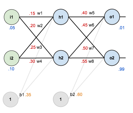
Overview : Here we use a neural network with two inputs, two hidden neurons, two output neurons. Additionally, the hidden and output neurons will include a bias. Here’s the basic structure:

In order to have some numbers to work with, here are the initial weights, the biases, and training inputs/outputs:

The goal of back propagation is to optimize the weights so that the neural network can learn how to correctly map arbitrary inputs to outputs. We will simulate with a single training set: given inputs 0.05 and 0.10, we want the neural network to output 0.01 and 0.99.

The Forward Pass : To begin, lets see what the neural network currently predicts given the weights and biases above and inputs of 0.05 and 0.10. To do this we’ll feed those inputs forward though the network.

We figure out the total net input to each hidden layer neuron, squash the total net input using an activation function (here we use the logistic function), then repeat the process with the output layer neurons.

Total net input is also referred to as just net input by some sources.

Here’s how we calculate the total net input for $h_1$ :

$net_{h1} = w_1 * i_1 + w_2 * i_2 + b_1 * 1$

$net_{h1} = 0.15 * 0.05 + 0.2 * 0.1 + 0.35 * 1 = 0.3775$

We then squash it using the logistic function to get the output of $h_1$ :

$out_{h1} = \frac{1}{1+e^{-net_{h1}}} = \frac{1}{1+e^{-0.3775}} = 0.593269992$

Carrying out the same process for $h_2$ we get:

$out_{h2} = 0.596884378$

We repeat this process for the output layer neurons, using the output from the hidden layer neurons as inputs.

Here’s the output for $o_1$ :

$net_{o1} = w_5 * out_{h1} + w_6 * out_{h2} + b_2 * 1$

$net_{o1} = 0.4 * 0.593269992 + 0.45 * 0.596884378 + 0.6 * 1 = 1.105905967$

$out_{o1} = \frac{1}{1+e^{-net_{o1}}} = \frac{1}{1+e^{-1.105905967}} = 0.75136507$

And carrying out the same process for $o_2$ we get:

$out_{o2} = 0.772928465$

Calculating the Total Error

We can now calculate the error for each output neuron using the squared error function and sum them to get the total error: $E_{total} = \sum \frac{1}{2}(target - output)^{2}$

The $\frac{1}{2}$ is included so that exponent is cancelled when we differentiate later on. The result is eventually multiplied by a learning rate anyway so it doesn’t matter that we introduce a constant here .

For example, the target output for $o_1$ is 0.01 but the neural network output 0.75136507, therefore its error is:

$E_{o1} = \frac{1}{2}(target_{o1} - out_{o1})^{2} = \frac{1}{2}(0.01 - 0.75136507)^{2} = 0.274811083$

Repeating this process for $o_2$ (remembering that the target is 0.99) we get:

$E_{o2} = 0.023560026$

The total error for the neural network is the sum of these errors:

$E_{total} = E_{o1} + E_{o2} = 0.274811083 + 0.023560026 = 0.298371109$

The Backwards Pass

Our goal with back propagation is to update each of the weights in the network so that they cause the actual output to be closer the target output, thereby minimizing the error for each output neuron and the network as a whole.

Output Layer

Consider $w_5$ . We want to know how much a change in $w_5$ affects the total error, aka $\frac{\partial E_{total}}{\partial w_{5}}$ .

$\frac{\partial E_{total}}{\partial w_{5}}$ is read as “the partial derivative of $E_{total}$ with respect to $w_{5}$ “. You can also say “the gradient with respect to $w_{5}$ “.

By applying the chain rule we know that:

$\frac{\partial E_{total}}{\partial w_{5}} = \frac{\partial E_{total}}{\partial out_{o1}} * \frac{\partial out_{o1}}{\partial net_{o1}} * \frac{\partial net_{o1}}{\partial w_{5}}$

Visually, here’s what we’re doing:

We need to figure out each piece in this equation.

First, how much does the total error change with respect to the output?

$E_{total} = \frac{1}{2}(target_{o1} - out_{o1})^{2} + \frac{1}{2}(target_{o2} - out_{o2})^{2}$

$\frac{\partial E_{total}}{\partial out_{o1}} = 2 * \frac{1}{2}(target_{o1} - out_{o1})^{2 - 1} * -1 + 0$

$\frac{\partial E_{total}}{\partial out_{o1}} = -(target_{o1} - out_{o1}) = -(0.01 - 0.75136507) = 0.74136507$

$-(target - out)$ is sometimes expressed as $out - target$

When we take the partial derivative of the total error with respect to $out_{o1}$ , the quantity $\frac{1}{2}(target_{o2} - out_{o2})^{2}$ becomes zero because $out_{o1}$ does not affect it which means we’re taking the derivative of a constant which is zero.

Next, how much does the output of $o_1$ change with respect to its total net input?

The partial derivative of the logistic function is the output multiplied by 1 minus the output:

$out_{o1} = \frac{1}{1+e^{-net_{o1}}}$

$\frac{\partial out_{o1}}{\partial net_{o1}} = out_{o1}(1 - out_{o1}) = 0.75136507(1 - 0.75136507) = 0.186815602$

Finally, how much does the total net input of $o1$ change with respect to $w_5$ ?

$net_{o1} = w_5 * out_{h1} + w_6 * out_{h2} + b_2 * 1$

$\frac{\partial net_{o1}}{\partial w_{5}} = 1 * out_{h1} * w_5^{(1 - 1)} + 0 + 0 = out_{h1} = 0.593269992$

Putting it all together:

$\frac{\partial E_{total}}{\partial w_{5}} = \frac{\partial E_{total}}{\partial out_{o1}} * \frac{\partial out_{o1}}{\partial net_{o1}} * \frac{\partial net_{o1}}{\partial w_{5}}$

$\frac{\partial E_{total}}{\partial w_{5}} = 0.74136507 * 0.186815602 * 0.593269992 = 0.082167041$

You’ll often see this calculation combined in the form of the delta rule:

$\frac{\partial E_{total}}{\partial w_{5}} = -(target_{o1} - out_{o1}) * out_{o1}(1 - out_{o1}) * out_{h1}$

Alternatively, we have $\frac{\partial E_{total}}{\partial out_{o1}}$ and $\frac{\partial out_{o1}}{\partial net_{o1}}$ which can be written as $\frac{\partial E_{total}}{\partial net_{o1}}$ , aka $\delta_{o1}$ (the Greek letter delta) aka the node delta. We can use this to rewrite the calculation above:

$\delta_{o1} = \frac{\partial E_{total}}{\partial out_{o1}} * \frac{\partial out_{o1}}{\partial net_{o1}} = \frac{\partial E_{total}}{\partial net_{o1}}$

$\delta_{o1} = -(target_{o1} - out_{o1}) * out_{o1}(1 - out_{o1})$

Therefore:

$\frac{\partial E_{total}}{\partial w_{5}} = \delta_{o1} out_{h1}$

Some sources extract the negative sign from $\delta$ so it would be written as:

$\frac{\partial E_{total}}{\partial w_{5}} = -\delta_{o1} out_{h1}$

To decrease the error, we then subtract this value from the current weight (optionally multiplied by some learning rate, eta, which we’ll set to 0.5):

$w_5^{+} = w_5 - \eta * \frac{\partial E_{total}}{\partial w_{5}} = 0.4 - 0.5 * 0.082167041 = 0.35891648$

Some sources use $\alpha$ (alpha) to represent the learning rate, others use $\eta$ (eta), and others even use $\epsilon$ (epsilon).

We can repeat this process to get the new weights $w_6$ , $w_7$ , and $w_8$ :

$w_6^{+} = 0.408666186$

$w_7^{+} = 0.511301270$

$w_8^{+} = 0.561370121$

We perform the actual updates in the neural network after we have the new weights leading into the hidden layer neurons (ie, we use the original weights, not the updated weights, when we continue the backpropagation algorithm below).

Hidden Layer

Next, we’ll continue the backwards pass by calculating new values for $w_1$ , $w_2$ , $w_3$ , and $w_4$ .

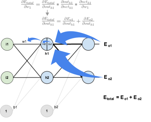
Big picture, here’s what we need to figure out:

$\frac{\partial E_{total}}{\partial w_{1}} = \frac{\partial E_{total}}{\partial out_{h1}} * \frac{\partial out_{h1}}{\partial net_{h1}} * \frac{\partial net_{h1}}{\partial w_{1}}$

Visually:

We’re going to use a similar process as we did for the output layer, but slightly different to account for the fact that the output of each hidden layer neuron contributes to the output (and therefore error) of multiple output neurons. We know that $out_{h1}$ affects both $out_{o1}$ and $out_{o2}$ therefore the $\frac{\partial E_{total}}{\partial out_{h1}}$ needs to take into consideration its effect on the both output neurons:

$\frac{\partial E_{total}}{\partial out_{h1}} = \frac{\partial E_{o1}}{\partial out_{h1}} + \frac{\partial E_{o2}}{\partial out_{h1}}$

Starting with $\frac{\partial E_{o1}}{\partial out_{h1}}$ :

$\frac{\partial E_{o1}}{\partial out_{h1}} = \frac{\partial E_{o1}}{\partial net_{o1}} * \frac{\partial net_{o1}}{\partial out_{h1}}$

We can calculate $\frac{\partial E_{o1}}{\partial net_{o1}}$ using values we calculated earlier:

$\frac{\partial E_{o1}}{\partial net_{o1}} = \frac{\partial E_{o1}}{\partial out_{o1}} * \frac{\partial out_{o1}}{\partial net_{o1}} = 0.74136507 * 0.186815602 = 0.138498562$

And $\frac{\partial net_{o1}}{\partial out_{h1}}$ is equal to $w_5$ :

$net_{o1} = w_5 * out_{h1} + w_6 * out_{h2} + b_2 * 1$

$\frac{\partial net_{o1}}{\partial out_{h1}} = w_5 = 0.40$

Plugging them in:

$\frac{\partial E_{o1}}{\partial out_{h1}} = \frac{\partial E_{o1}}{\partial net_{o1}} * \frac{\partial net_{o1}}{\partial out_{h1}} = 0.138498562 * 0.40 = 0.055399425$

Following the same process for $\frac{\partial E_{o2}}{\partial out_{h1}}$ , we get:

$\frac{\partial E_{o2}}{\partial out_{h1}} = -0.019049119$

Therefore:

$\frac{\partial E_{total}}{\partial out_{h1}} = \frac{\partial E_{o1}}{\partial out_{h1}} + \frac{\partial E_{o2}}{\partial out_{h1}} = 0.055399425 + -0.019049119 = 0.036350306$

Now that we have $\frac{\partial E_{total}}{\partial out_{h1}}$ , we need to figure out $\frac{\partial out_{h1}}{\partial net_{h1}}$ and then $\frac{\partial net_{h1}}{\partial w}$ for each weight:

$out_{h1} = \frac{1}{1+e^{-net_{h1}}}$

$\frac{\partial out_{h1}}{\partial net_{h1}} = out_{h1}(1 - out_{h1}) = 0.59326999(1 - 0.59326999 ) = 0.241300709$

We calculate the partial derivative of the total net input to $h_1$ with respect to $w_1$ the same as we did for the output neuron:

$net_{h1} = w_1 * i_1 + w_3 * i_2 + b_1 * 1$

$\frac{\partial net_{h1}}{\partial w_1} = i_1 = 0.05$

Putting it all together:

$\frac{\partial E_{total}}{\partial w_{1}} = \frac{\partial E_{total}}{\partial out_{h1}} * \frac{\partial out_{h1}}{\partial net_{h1}} * \frac{\partial net_{h1}}{\partial w_{1}}$

$\frac{\partial E_{total}}{\partial w_{1}} = 0.036350306 * 0.241300709 * 0.05 = 0.000438568$

You might also see this written as:

$\frac{\partial E_{total}}{\partial w_{1}} = (\sum\limits_{o}{\frac{\partial E_{total}}{\partial out_{o}} * \frac{\partial out_{o}}{\partial net_{o}} * \frac{\partial net_{o}}{\partial out_{h1}}}) * \frac{\partial out_{h1}}{\partial net_{h1}} * \frac{\partial net_{h1}}{\partial w_{1}}$

$\frac{\partial E_{total}}{\partial w_{1}} = (\sum\limits_{o}{\delta_{o} * w_{ho}}) * out_{h1}(1 - out_{h1}) * i_{1}$

$\frac{\partial E_{total}}{\partial w_{1}} = \delta_{h1}i_{1}$

We can now update $w_1$ :

$w_1^{+} = w_1 - \eta * \frac{\partial E_{total}}{\partial w_{1}} = 0.15 - 0.5 * 0.000438568 = 0.149780716$

Repeating this for $w_2$ , $w_3$ , and $w_4$

$w_2^{+} = 0.19956143$

$w_3^{+} = 0.24975114$

$w_4^{+} = 0.29950229$

Finally, we’ve updated all of our weights! When we fed forward the 0.05 and 0.1 inputs originally, the error on the network was 0.298371109. After this first round of back propagation, the total error is now down to 0.291027924. It might not seem like much, but after repeating this process 10,000 times, for example, the error plummets to 0.0000351085. At this point, when we feed forward 0.05 and 0.1, the two outputs neurons generate 0.015912196 (vs 0.01 target) and 0.984065734 (vs 0.99 target).

MY BLOGS

Wednesday 12 December 2018

VTU PYTHON SYLLABUS

Wednesday 7 November 2018

List of Machine Learning Algorithms

1. Find S Algorithm

2. List then Elimination Algorithm

Saturday 22 September 2018

A Step by Step Backpropagation Example

Reference : https://mattmazur.com/2015/03/17/a-step-by-step-backpropagation-example/

Overview : Here we use a neural network with two inputs, two hidden neurons, two output neurons. Additionally, the hidden and output neurons will include a bias. Here’s the basic structure:

The Forward Pass : To begin, lets see what the neural network currently predicts given the weights and biases above and inputs of 0.05 and 0.10. To do this we’ll feed those inputs forward though the network.

Calculating the Total Error

The Backwards Pass

Output Layer

Hidden Layer

Activation function in Neural network

Back Propagation in Neural Network

Explained In A Minute: Neural Networks

Machine Learning for Flappy Bird using Neural Network & Genetic Algorithm

Neural Networks Explained - Machine Learning Tutorial for Beginners